Visualizing a 3-D volume with napari

A reconstructed 3-D ultrasound volume can be visualized with napari. Before visualization, the beamformed volume is converted to a B-mode display volume, clipped in dB, and normalized between 0 and 1.

Napari is an optional external viewer and is not required by UltraSpy.

import numpy as np
import napari

def window_db_volume(volume, db_min=-55, db_max=0, ref_value=None):
    """Prepare a 3-D beamformed volume for visualization with napari."""
    volume = np.abs(volume).astype(np.float32)

    if ref_value is None:
        ref_value = np.max(volume)

    if ref_value <= 0:
        ref_value = 1.0

    volume = volume / ref_value
    volume = np.maximum(volume, np.finfo(np.float32).eps)

    volume_db = 20 * np.log10(volume)
    volume_db = np.clip(volume_db, db_min, db_max)

    return ((volume_db - db_min) / (db_max - db_min)).astype(np.float32)


# x, y and z are the physical coordinates used to build the GridScan.
# They are usually defined in meters in UltraSpy, for example:
#
# x = np.linspace(-5.0, 5.0, nx, dtype=np.float32) * 1e-3
# y = np.linspace(-5.0, 5.0, ny, dtype=np.float32) * 1e-3
# z = np.linspace(5.0, 35.0, nz, dtype=np.float32) * 1e-3
#
# The reconstructed volume follows the same axis order as the scan:
# beamformed_volume[x, y, z].

vol_display = window_db_volume(beamformed_volume, db_min=-55, db_max=0)

# Napari expects image arrays in display order [Z, Y, X]. If the UltraSpy
# volume is stored as [X, Y, Z], move the axes before adding it to napari.
vol_display_zyx = np.transpose(vol_display, (2, 1, 0))

# The scale gives the voxel spacing in the same order as the displayed
# array. The coordinates are converted from meters to millimeters here so
# napari displays physical distances in mm.
dz_mm = float((z[1] - z[0]) * 1000) if len(z) > 1 else 1.0
dy_mm = float((y[1] - y[0]) * 1000) if len(y) > 1 else 1.0
dx_mm = float((x[1] - x[0]) * 1000) if len(x) > 1 else 1.0

viewer = napari.Viewer()

viewer.add_image(
    vol_display_zyx,
    name="B-mode volume",
    scale=(dz_mm, dy_mm, dx_mm),
    colormap="gray",
    contrast_limits=(0, 1),
    rendering="mip",
    axis_labels=["Z", "Y", "X"],
)

napari.run()

Example output

The reconstructed 3-D B-mode volume can then be explored interactively in napari. The viewer allows the user to inspect the volume slice by slice or to display it using a 3-D rendering mode such as maximum intensity projection (MIP).

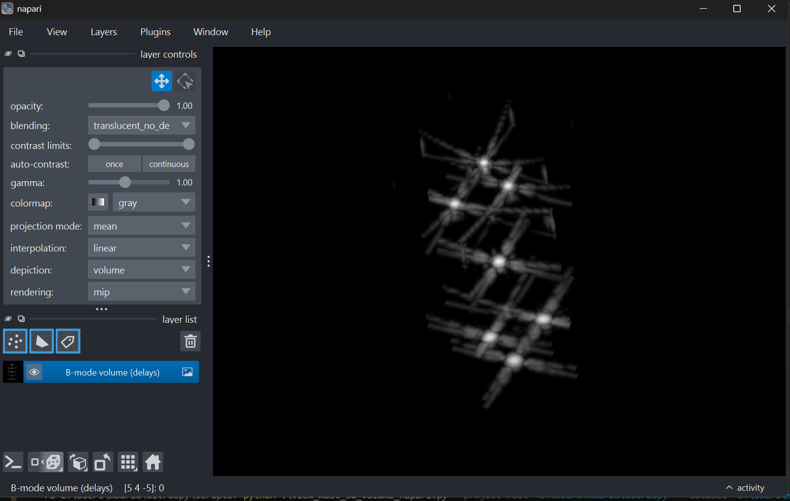
Example of a reconstructed 3-D B-mode ultrasound volume displayed with napari using a maximum intensity projection rendering.