Use of metrics

This tutorial will show how to use the metrics methods in our data. We highly recommend you to follow at the very least the DAS before starting this one.

Well, let’s start! First, we will compute the Signal Noise to Ratio (SNR) of a data file we’ve acquired using the system from the company DB-SAS (PA2). Note that the metrics module is only implemented on CPU.

from ultraspy.io.reader import Reader

reader = Reader('/path/to/pa2_wire.mat', 'dbsas')
first_frame = reader.data[0]

In order to compute the SNR of our signals, we first need to define where to find both the pulse and the noise. It is hard to automate this efficiently, so it’s better if the user can define these boundaries by himself, but if he doesn’t, we also provide a function to return the most salient point of a set of data which is based on the data time sample which received the highest intensity. In the case of our data, if we display it, we see that there are a lot of echoes close to the probe, and it will seriously affect the detection of the most salient point.

import matplotlib.pyplot as plt

# Raw signals before pre-processing
plt.imshow(first_frame[0], aspect='auto', clim=[0, 1000])
plt.title('Raw data')
plt.show()

As we can see, the echoes are very strong close to the probe, so if we try to detect the most salient point on all the data, the coordinates wont be correct. From the previous graph, we can estimate that the first thousand time samples can be ignored in order to correctly estimate the position of the most salient point. The metrics module has a method to estimate the position of the signal and the noise:

# The metrics are on CPU only
import ultraspy as us

# Try to define the signal and noise boundaries for the 64th probe element
# (middle of the probe). Also note the call using .cpu to access the CPU
# methods
bounds = us.metrics.find_signal_and_noise(first_frame[0, 64], show=True)

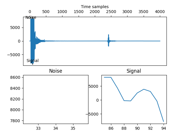
Definitely, the bounds are incorrect because the signal has been detected in the echoes at the beginning of the signal. However, if we estimate that we can ignore the first thousand time samples we get:

# Same, but skipping the first 1000 time samples
bounds = us.metrics.find_signal_and_noise(first_frame[0, 64],
                                          ignore_until=1000, show=True)

Much better! Also note that the option show=True can be set in most of the metrics methods in order to visualize if the automatic assumptions are correctly made. Here we can clearly see the pulse of the wire, which has been quite correctly picked, and the noise is quite ok as well, so we’ll use these boundaries to compute the SNR. A few options can be updated in the find_signal_and_noise method, such as the ignore_until if the boundaries don’t fit. If you want to use your own boundaries (which is recommended), you can use the following arguments (more information in the API reference):

snr = us.metrics.signal_noise_ratio(first_frame[0, 64], *bounds)
print(f'SNR: {snr}')

SNR: 49.73140340436306

Nice! That’s an okay value considering we didn’t do any pre-processing on our data. Indeed, despite the data we’ve used in the previous tutorials, those are experimental, coming from a real echograph. Every system have its own data format, and its own pros and cons, so it is a bit hard here to be provide an exhaustive list of things to think about when processing new data. However, most of the time, it is a good practice to apply a band-pass filter on data. Let’s check in practice how to apply such filter and how it affects the SNR.

GPU versionCPU version

import numpy as np
import cupy as cp

# The central frequency of the probe was ~5MHz, so a band-pass
# filter between 2 and 8MHz should provide good results
sampling_freq = reader.acquisition_info['sampling_freq']
d_filtered = cp.asarray(first_frame.copy(), np.float32)
us.filtfilt(d_filtered, 2e6, sampling_freq, 'high')
us.filtfilt(d_filtered, 8e6, sampling_freq, 'low')
filtered = d_filtered.get()

# Let's check the SNR of the filtered data
snr = us.metrics.signal_noise_ratio(filtered[0, 64], *bounds)
print(f'SNR: {snr}')

SNR: 54.3275968698127

Well, that’s quite explicit! A simple filter improved the SNR by almost 5dB. We also can visualize the spectra of the raw and filtered data to understand a bit more how the signal has been improved:

sampling_freq = reader.acquisition_info['sampling_freq']
frequencies, spectrum_raw = us.cpu.get_spectrum(first_frame[0], sampling_freq)
_, spectrum_filtered = us.cpu.get_spectrum(filtered[0], sampling_freq)
frequencies *= 1e-6  # Convert to MHz

fig, axes = plt.subplots(1, 2)
extent = [frequencies[0], frequencies[-1], 128, 1]
axes[0].imshow(spectrum_raw, aspect='auto', clim=[-40, 0], extent=extent)
axes[0].set_xlabel('Frequencies (MHz)')
axes[0].set_ylabel('Probe elements')
axes[0].set_title('Spectra of raw data')
im2 = axes[1].imshow(spectrum_filtered, aspect='auto', clim=[-40, 0], extent=extent)
axes[1].set_xlabel('Frequencies (MHz)')
axes[1].set_title('Spectra of filtered data')
fig.colorbar(im2, ax=axes[1])
plt.show()

You can see in axis the frequencies (in MHz). The central frequency of the L7-4 probe is 5.208MHz, which is clearly the dominant frequency in the spectrum. However, we also can see that the signal is pretty noisy. However, on the filtered spectra in the image on the right, the band of interest is much more preserved.

Let’s now compute the metrics on beamformed images. For that, we need to perform the beamforming first.

import numpy as np
from ultraspy.scan import GridScan
from ultraspy.beamformers.das import DelayAndSum

# Let's do everything on CPU, for simplicity
beamformer = DelayAndSum(on_gpu=False)
beamformer.automatic_setup(reader.acquisition_info, reader.probe)
beamformer.update_setup('f_number', 1.)
beamformer.update_setup('sound_speed', 1450)
beamformer.update_setup('signal_duration', 0.6 * 1e-6)
x = np.linspace(-15, 15, 500) * 1e-3
z = np.linspace(20, 70, 1000) * 1e-3
scan = GridScan(x, z)

# Beamforming, then compute the envelope of the beamformed signal
output = beamformer.beamform(first_frame, scan)
envelope = beamformer.compute_envelope(output, scan)
b_mode = us.cpu.to_b_mode(envelope)

There we go, now we have the b-Mode to evaluate, you can visualize it using the sample of code we saw in previous tutorials if you want. The first metrics to evaluate here are the ones related to the envelope lobes: the FWHM and PSL. As for the SNR, we need to know where the lobe of interest is. It is very high-level information, but we’ll suppose here that it is simply the maximum value of the B-Mode:

focus_point = us.metrics.get_most_salient_point(b_mode)
lobe_metrics = us.metrics.get_lobe_metrics(b_mode, focus_point, x, z, show=True)
print("Lateral:\n"
      f"\tFWHM: {lobe_metrics['lateral_fwhm']}\n"
      f"\tPSL: {lobe_metrics['lateral_psl']}\n"
      "Axial:\n"
      f"\tFWHM: {lobe_metrics['axial_fwhm']}\n"
      f"\tPSL: {lobe_metrics['axial_psl']}\n")

Lateral:
    FWHM: 0.0004884134687981584
    PSL: 19.682097908267608
Axial:
    FWHM: 0.0003490619581923496
    PSL: 30.315017735741883

The last metric we want to show here is the CNR, based on contrast study. However, there is no point to visualize it with the wire data, as there aren’t much contrast to observe. Instead, we’ll do it on the rotating disk we saw in the Doppler tutorial. First we need to recover the new b-Mode:

reader = Reader('/path/to/rotating_disk.mat', 'must')
first_frame = reader.data[0]

# Adjust our beamformer, no need to create a new one
beamformer.set_is_iq(True)
beamformer.automatic_setup(reader.acquisition_info, reader.probe)
beamformer.update_setup('signal_duration', 0)
x = np.linspace(-12.5, 12.5, 250) * 1e-3
z = np.linspace(10, 35, 250) * 1e-3
scan = GridScan(x, z)

# We're working on I/Qs
info = beamformer.setup
iqs = us.cpu.rf2iq(first_frame, info['central_freq'], info['sampling_freq'],
                   beamformer.t0)
output = beamformer.beamform(iqs, scan)
envelope = beamformer.compute_envelope(output, scan)
b_mode = us.cpu.to_b_mode(envelope)

For the CNR, we need to define where are the areas to observe (typically the cysts or equivalent). To do that, we provide an utility function to build masks of miscellaneous shapes (circles, empty circles, or rectangles). ultraspy expects a mask for both signal and noise. Let’s build these masks first:

# We define the area of interest. Here a circle is good as we are willing
# to observe the rotating disk. Since we know its center and radius (in mm)
# it is easy to build its mask:
center = (-1e-3, 22.5e-3)
disk_radius = 10e-3
disk_mask = us.metrics.build_mask(center, disk_radius, x, z, 'circle')

# Then we define a noise area, here an empty circle seems good, as it will
# be as close as possible to our interest area. It could also be a
# rectangle or whatever tho.
noise_radius = 12.5e-3
noise_offset = 2e-3
noise_mask = us.metrics.build_mask(center, (noise_radius, noise_offset),
                                   x, z, 'empty_circle')

If we want to visualize the masks, we can use the following script and make sure we’ve selected them properly:

import matplotlib.pyplot as plt

extent = [x * 1e3 for x in [x[0], x[-1], z[-1], z[0]]]  # In mm
b_mode_args = {'extent': extent, 'cmap': 'gray', 'clim': [-60, 0]}
fig, axs = plt.subplots(1, 3)
axs[0].imshow(b_mode.T, **b_mode_args)
axs[1].imshow(np.ma.masked_where(disk_mask, b_mode.T), **b_mode_args)
axs[2].imshow(np.ma.masked_where(noise_mask, b_mode.T), **b_mode_args)
plt.show()

Looks good! So we can use them to compute our CNR:

cnr = us.metrics.get_contrat_noise_ratio(b_mode.T, disk_mask, noise_mask)
print(f'CNR: {cnr}')

CNR: 8.11761872362058